Okay, this was course work so I won’t go into too much details about what the game was or how exactly the code was written (We wouldn’t want anyone to just copy it right 😉 ), but I’ll go over the concepts introduced. I had so much fun working on this 😄
The Game
Essentially it’s a made-up two-player board game, where each player aims at eliminating all the opponent player’s pieces. The constraint is that every AI move must be selected in under 3 seconds. At each turn, the AI must decide what the best move is for the current player.
MiniMax
First I generate a tree where the root node is the current game state. Then the children are all the possible game states that can be created from the current one, given that only the current player can make a move. Then we switch turns and keep generating children recursively (using depth-first). We can go on forever (until we’ve reached endgames) but of course… ain’t nobody got time fo’ dat! We only have 3 seconds. So I set a constant depth limit of 3 levels down the tree for example where the search tree stops expanding.
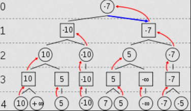
Now we implement something called mini-max. After evaluating the leaf nodes of the tree (we’ll talk about evaluation later), the values need to be propagated up the tree until only one remains and the next move is picked (bottom-up). To do that, we assume that the player who’s turn it is (levels 0-2-4 in the image below) will always try to maximize the outcome, while their opponent (levels 1-3-etc.) will always try to minimize the result for the max player’s move. So at each level, the nodes will pick from their children the one that is either the maximum (for max’s level) or minimum (for min’s level) of all children.

Alpha-Beta Pruning
Problem
Cool! But sometimes parts of the tree are irrelevant to evaluate and can be cut out to save time, in the case where there’s no chance that a maximizing (or minimizing) node would ever even consider to choose them.
Solution
That happens a lot and it is called alpha-beta pruning. You can visualize alpha-beta (and minimax) on the following link courtesy of the University of Berkeley: http://inst.eecs.berkeley.edu/~cs61b/fa14/ta-materials/apps/ab_tree_practice/
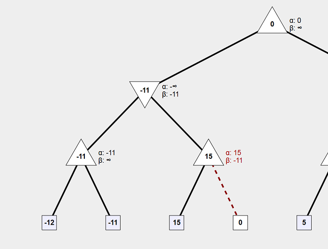
Let’s take a closer look at the following image. We can see that a branch has been pruned because its value will not change the result that will eventually be brought up. If the value is less than the value of the parent node, 15, (yes we see that it is, but we theoretically haven’t calculated it at this point; we are going depth-first), then the max node (parent) will not select it. If that value is more than the value of the parent node, that still doesn’t matter because the parent’s parent (the min node above), will never select a value higher than -11 because it wants to minimize the result. So that branch is pruned; no matter what its value is it will not be useful.

Note: If the branching factor at that node was more than 2, then every one of the extra branches would also have been pruned.
Iterative Deepening
Another Problem…
We now have the ability to go deeper down the tree in the same amount of time, because parts of the tree are completely ignored. But we still have another problem though… or lack of efficient resource usage. Depending on the game state, sometimes there are more children to explore and thus the tree is way wider (higher branching factor). This means that it takes more time to go to the same depth and keeping a constant depth to explore throughout the whole game is not efficient. At depth level 3 for example the average execution time is 0.2 seconds, with no move using more than 3 seconds. Sometimes depth 4 takes 0.3 seconds, which is awesome, but at certain game states it takes 11 seconds to go down to the same level. That’s a huge discrepancy and you want to make sure you always use the amount of time you are given (3 seconds) without exceeding it and without underusing it either (the deeper you go the more informed your decision is).
Solution
To solve this, you can sometimes go deeper in order to use up to 3 seconds, and sometimes you need to cut it short because continuing to a certain depth means it’ll take too long to compute. So basically adapt the explored depth based on the game state, and I do that with a technique called iterative deepening.
Iterative deepening is basically depth-first search, but with an increasing depth limit. We start our search at a depth limit of 1, and once we are done we increment the depth level and start the search again. Keep in mind that the children of previously explored nodes will not change if they have already been generated, so the actual time it takes for iterative deepening isn’t that much worse than exploring a fixed depth, especially if your evaluation function isn’t too expensive. I add a timer to ensure the threshold of 3 seconds is never broken. When the allocated time runs out, whatever value we have brought up last can be selected right away. The result is that the depth increases as the branching factor lowers and we are left with a varying depth explored over the course of a match. This for obvious reasons was a game-changer, maximizing the time resource while exploring deeper levels overall. The image below is a small sample of the time in seconds for a decision to be made at each turn, and the depth-level explored at that turn. An average of 5 levels explored over the course of a game!

Note: The average execution time is always around 2.85 seconds because that was my hard limit to make sure that 3 seconds will never ever be surpassed (better safe than sorry 😌).
Depth-Preferred Transposition Table
I mentioned that we can keep the children in memory with iterative deepening to avoid having to regenerate them, but we also have the possibility of encountering the same game state multiple times in the same tree. So we can save the calculated value of a node in order to reuse it if needed. For this we use a depth-preferred transposition table. A calculated value that is further away from a leaf node (higher up the tree relative to the depth explored) is preferred because its value is more informed, it is brought up from a longer chain of events. This allows us the possibility of having a leaf node informed to lower depths that technically haven’t been visited but can simply be replayed. We know that the children of a given game state will always be the same if it is the same player’s turn.
Heuristic - Evaluation Function
Finally, you know that “calculated value” that we have been bringing up the tree this whole time? Well that’s called the heuristic value which is found by running the heuristic function at a game state. The Heuristic function is the actual algorithm that calculates how good or bad a given game state is. It runs on our terminal nodes (tree leaves), wherever they may be. This is 100% dependent on the actual game so it’ll be useless to explain my heuristic without knowing how the game works exactly. But for a heuristic to be good it requires a deep analysis and understanding about how the game works, what positions are better/weaker and what tactics are beneficial over time.
Conclusion
Anyways I had so much fun working on this. Part of the reason why this was so exciting for me is that I play Chess all the time (seriously, every single day) and now that I have researched and implemented my own system, I understand how chess AI players work. Of course top board game AIs do way more advanced stuff that you can read all about online, but knowing the building blocks behind something you use every day is really awesome!
I was hoping to keep this as short as possible, so I tried to simplify things a bit (How did that work out? 😬).
Since you made it this far… have a wonderful day 😊